Does a Histogram Reflect Continuous Quantitative Data

Objectives

By the end of this section, you will be able to...

1. construct bar graph
2. construct pie charts
3. construct histograms for discrete and continuous data
4. draw stem-and-leaf plots
5. draw dot plots
6. identify the shape of a distribution
7. construct frequency polygons*
8. construct ogives*
9. draw time-series graphs

* You will not be tested on these objectives.

For a quick overview of this section, watch this short video summary:

Bar Graphs

Bar graphs are probably the most commonly used graphs, and one you're already familiar with. I won't mention much more here, except to state a couple keys:

1. heights can be frequency or relative frequency
2. bars must not touch

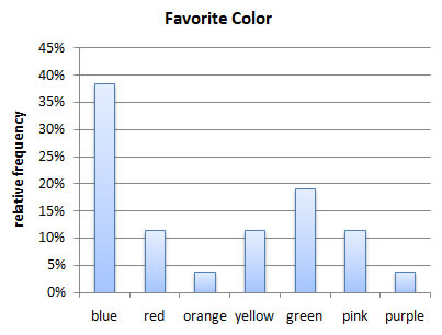
Using our the data from our previous color example,

favorite color	frequency	relative frequency
blue	10	10/26 ≈ 0.38
red	3	3/26 ≈ 0.12
orange	1	1/26 ≈ 0.04
yellow	3	3/26 ≈ 0.12
green	5	5/26 ≈ 0.19
pink	3	3/26 ≈ 0.12
purple	1	1/26 ≈ 0.04

we could then make both frequency and relative frequency bar graphs.

Technology

Here's a quick overview of how to create bar graphs in StatCrunch.

1. Enter or import the data.
2. Select Graphics > Bar Graph, then choose with data or with summary.
3. If you chose with data, select the column(s) you wish to use and click Next. If you chose with summary, set the columns containing the categories and counts and click Next.
4. Choose the type (Frequency or Relative Frequency) and click Next.
5. Enter any modifications and/or color schemes and click Create Graph!
6. You can then choose Options > Copy to copy the box plot for use elsewhere.

Pareto Charts

A Pareto chart is a bar graph whose bars are drawn in decreasing order of frequency or relative frequency.

You see Pareto charts fairly often in the newspaper, because often the article is trying to show that one particular category is the highest or lowest. The image below, for example, is from the Chicago Tribune. You can see clearly from the graph that it's attempting to show that the local BP refinery in Whiting, Indiana is the highest-capacity refinery that is considering expansion.

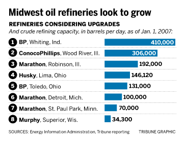
If you don't remember the issue, you can read up about BP's plan to expand it's refinery in this article from CBS2 Chicago.

Here's another one, using the favorite color data from the last section:

Side-by-Side Bar Graphs

Side-by-side bar graphs are used when you want to compare two different populations. The key with side-by-side bar graphs is that you must use relative frequencies. Do you know why?

I think so. But just in case...

Look at it this way: Let's suppose we want to compare the poverty levels for different cities in Illinois. If we used frequencies only, Cook county dominates - almost 800,000, where no other county has over 50,000. On the other hand, if we looked at relative frequency, Cook county still has the most (15%), but other counties such as Kane are close, with rates around 8%.

Source: 2007 Illinois Poverty Summit

Here's a good example of a side-by-side chart, from the Associated Press.

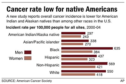
What's shown isn't quite a relative frequency as we've defined it - it's the number per 100,000, where ours as a percent is the number per 100. The reason why the rate per 100,000 is used here is because the percents would all be less than 1% and difficult to read. Still, if frequency was used instead, the "White" category would be the largest, simply because that's the largest segment of the U.S. population.

Technology

Here's a quick overview of how to create side-by-side bar graphs in StatCrunch.

1. Enter or import the data.
2. Select Graphics > Chart > Columns
3. Select the columns you'll be using.
4. Select the location of the lablels (Row labels in).
5. If desired, choose an order.
6. Choose the plot type (vertical bars for a side-by-side bar graph) and click Next.
7. Enter any modifications and/or color schemes and click Create Graph!
8. You can then choose Options > Copy to copy the box plot for use elsewhere.

Pie Charts

Like bar graphs, pie charts are very common. You're probably already aware of these as well. I'll just include a couple comments:

1. should always include the relative frequency
2. also should include labels, either directly or as a legend

Using our the data from our previous color example,

favorite color	frequency	relative frequency
blue	10	10/26 ≈ 0.38
red	3	3/26 ≈ 0.12
orange	1	1/26 ≈ 0.04
yellow	3	3/26 ≈ 0.12
green	5	5/26 ≈ 0.19
pink	3	3/26 ≈ 0.12
purple	1	1/26 ≈ 0.04

we get this pie chart:.

Technology

Here's a quick overview of how to create pie charts in StatCrunch.

1. Enter or import the data.
2. Select Graphics > Pie Chart, then choose with data or with summary.
3. If you chose with data, select the column(s) you wish to use and click Next. If you chose with summary, set the columns containing the categories and counts and click Next.
4. Enter any modifications (labels, title, color scheme, etc) and click Create Graph!
5. You can then choose Options > Copy to copy the box plot for use elsewhere.

Histograms

Histograms are so important that they got their own video!

Single-valued Histograms

To display quantitative data, we need a new type of chart, called a histogram. Histograms look similar to bar graphs, but they have some distinct differences - and for good reason.

A histogram is constructed by drawing rectangles for each class of data. The height of each rectangle is the frequency or relative frequency of the class. The width of each rectangle is the same and the rectangles touch each other.

The rectangles need to touch in a histogram because we want to imply that the classes are adjacent. In a bar graph, a favorite color of "blue" isn't really adjacent to "red", even though we might put it that way in a bar graph. For quantitative data like the data used in Example 1 earlier this section, the value 2 really is next to the value 3.

Let's take a closer look at that example.

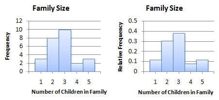
Example 4

children	frequency	relative frequency
1	3	3/26 ≈ 0.12
2	8	8/26 ≈ 0.31
3	10	10/26 ≈ 0.38
4	2	2/26 ≈ 0.08
5	3	3/26 ≈ 0.12

To make a histogram, we make what looks like a bar graph with a couple key differences:

1. rectangles must touch
2. class labels are underneath the rectangle

Here's what they'd look like for our example data:

Technology

Here's a quick overview of how to create histograms for single-valued discrete data using StatCrunch.

1. Enter or import the data.
2. Select Graphics > Histogram
3. Select the column(s) you want to summarize and click Next.
4. Set the Type , lower class limit (Start bins at:).
5. Set the class width (bin) to 1, and click Calculate.

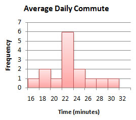
Histograms for Multi-valued and Continuous Data

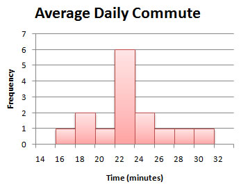
Multi-valued and continuous histograms are probably where the most errors occur. There are some key differences between this and single-valued histograms. In this case, each rectangle doesn't represent a single value, but rather a range of values. Because of that, we don't label the class on the horizontal axis. Instead, we label the lower class limits at the left edge of each rectangle.

Let's demonstrate using an example:

Example 5

average commute	frequency	relative frequency
16-17.9	1	1/15 ≈ 0.07
18-19.9	2	2/15 ≈ 0.13
20-21.9	1	1/15 ≈ 0.07
22-23.9	6	6/15 = 0.40
24-25.9	2	2/15 ≈ 0.13
26-27.9	1	1/15 ≈ 0.07
28-29.9	1	1/15 ≈ 0.07
30-31.9	1	1/15 ≈ 0.07

Here's what a frequency histogram would look like for these data:

Technology

Here's a quick overview of how to create histograms for multi-valued discrete data or continuous data in StatCrunch.

1. Enter or import the data.
2. Select Graphics > Histogram
3. Select the column(s) you want to summarize and click Next.
4. Set the Type, lower class limit (Start bins at:), and class width (bin), then click Calculate.

One final note about histograms: Because they show us such nice information about the distribution of a set of data, we'll be using them frequently throughout the rest of the semester. Be sure you spend plenty of time familiarizing yourself with the technology, so you're able to create histograms with ease.

Stem-and-Leaf Plots

Stem-and-leaf plots are another way to represent quantitative data. They give more detail because they show the actual data. The idea is to split each data value into two parts - a stem and a leaf. The stem is everything of the right-most digit, and the leaf is that right-most digit. Here's an example, using the data from earlier this section regarding exam scores from a previous Mth120 class.

Example 6

62	87	67	58	95	94	91	69	52
76	82	85	91	60	77	72	83	79
63	88	79	88	70	75	87

With these data, the stems are the first digits - 5, 6, 7, 8, and 9. The leafs are all the second digits, 0, 1, ... , 9. The full stem-and-leaf plot lists the stems down the left side, a vertical bar between, and then lists the leafs in order to the right. Something like this:

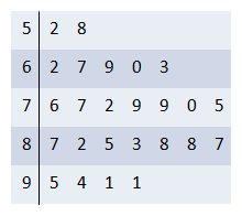
It's interesting that this plot looks very similar to a histogram, only it gives us the actual data. Take a look at this animation to see the relationship:

There are some limitations to stem-and-leaf plots. In particular, we're limited to small data sets - can you imagine the leaves if we had 1,000 test scores? Also, the range in the data needs to be fairly small.

By that, I mean if the data values range from 1-100, our stems can be 0, 10, 20, ... , 90, as they were in this example. On the other hand, if the values range from 1-10,000, the stems would have to be 0, 10, 20, ... , 9,980, 9,990. That's a lot of rows!

Technology

Here's a quick overview of how to create stem-and-leaf plots in StatCrunch.

1. Enter or import the data.
2. Select Graphics > Stem and Leaf
3. Select the column you wish to use and click Create Graph!

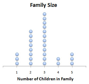
Dot Plots

Dot pots are similar to single-valued histograms, but rather than placing rectangles above each particular value, a dot plot just places the required number of dots above each value. Looking at our example again with the number of children, the plot would look something like this:

Technology

Here's a quick overview of how to create dot plots in StatCrunch.

1. Enter or import the data.
2. Select Graphics > Dotplot.
3. Select the column you wish to use and click Next.
4. Set any options and click Create Graph!

Distribution Shape

A good way to describe a distribution is its shape. In general, we describe a distribution's shape in one of four ways (though there are others):

1. uniform - frequencies are evenly spread out among all values of the variable
2. symmetric (bell-shaped) - highest value is in the middle, with values tailing off to the right and left
3. left (negative) skewed - highest value is on the right, with a longer left "tail"
4. right (positive) skewed - highest values is on the left, with a longer right "tail"

In addition to histograms, stem-and-leaf plots, and dot plots, there are some other, section common plots. We'll introduce a couple in this section. The first type, frequency polygons, are not a type of plot that will be expected of you on exams, though you will be asked questions about them on homework.

Frequency Polygons

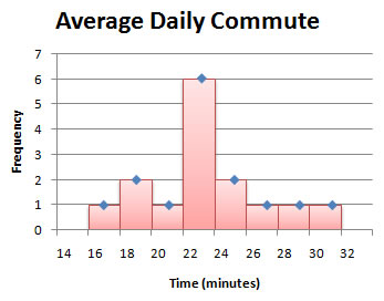
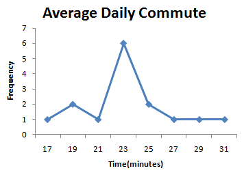
A frequency polygon is drawn by plotting a point above each class midpoint and connecting the points with a straight line. (Class midpoints are found by average successive lower class limits.)

Example 1

To illustrate the idea, let's look at the average commute data from the last section.

average commute	midpoint	frequency	relative frequency
16-17.9	17	1	1/15 ≈ 0.07
18-19.9	19	2	2/15 ≈ 0.13
20-21.9	21	1	1/15 ≈ 0.07
22-23.9	23	6	6/15 = 0.40
24-25.9	25	2	2/15 ≈ 0.13
26-27.9	27	1	1/15 ≈ 0.07
28-29.9	29	1	1/15 ≈ 0.07
30-31.9	31	1	1/15 ≈ 0.07

The three images below show the relationship between the histogram and the frequency polygon.

Note: No technology section this time, since you won't be asked to do this for exams.

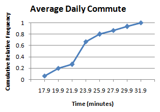
Ogives

Ogives are pretty funky graphs, and rarely used except in specific areas. We'll just give a quick example here, but like frequency polygons, you won't be expected to create these on an exam. (Though it may come up in homework.)

An ogive (read as "oh jive") is a graph that represents the cumulative frequency or cumulative relative frequency for the class. It is constructed by plotting points - the x-coordinates are the upper class limits and the y-coordinate is the corresponding cumulative frequency or cumulative relative frequency.

Example 3

To illustrate the idea, let's again use the average commute data from the last section.

average commute	relative frequency	cumulative relative frequency
16-17.9	1/15 ≈ 0.07	1/15 ≈ 0.07
18-19.9	2/15 ≈ 0.13	3/15 ≈ 0.20
20-21.9	1/15 ≈ 0.07	4/15 ≈ 0.27
22-23.9	6/15 = 0.40	10/15 ≈ 0.67
24-25.9	2/15 ≈ 0.13	12/15 = 0.80
26-27.9	1/15 ≈ 0.07	13/15 ≈ 0.87
28-29.9	1/15 ≈ 0.07	14/15 ≈ 0.93
30-31.9	1/15 ≈ 0.07	15/15 = 1.00

Note: No technology section this time, since you won't be asked to do this for exams.

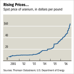
Time-Series Graphs

Time series graphs are much more common than the last couple times we've looked at. It's common to see stock prices and daily temperature graphs in the news - both are time series plots.

A time series plot is obtained by plotting the time in which a variable is measured on the horizontal axis and the corresponding value of the variable on the vertical axis.

The example above is from the Chicago Tribune and reflects the price of uranium from 2001-2006.

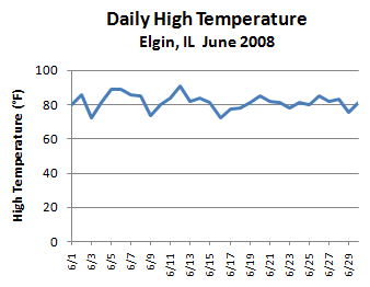
Example 4

Here's another example, using the daily high temperature in Elgin, IL, for the month of June, 2008.

date	daily high temperature
6/1	80
6/2	86
6/3	72
6/4	81
6/5	89
6/6	89
6/7	86
6/8	85
6/9	73
6/10	80
6/11	84
6/12	91
6/13	82
6/14	84
6/15	81
6/16	72
6/17	77
6/18	78
6/19	81
6/20	85
6/21	82
6/22	81
6/23	78
6/24	81
6/25	80
6/26	85
6/27	82
6/28	83
6/29	75
6/30	81

And the time series plot would look something like this:

Technology

Here's a quick overview of how to create a time series plot in StatCrunch.

1. Enter or import the data.
2. Select Graphics > Index Plot
3. Select the column(s) you want to plot and click Next.
4. Set any desired options and click Create Graph!

sharkeyagoorgurnote.blogspot.com

Source: https://faculty.elgin.edu/dkernler/statistics/ch02/2-2.html

Share this post